
The following is a description of the workflow that we use at the ChEAS (Chequamegon Ecosystem-Atmosphere Study) core-site cluster based at the University of Wisconsin to create real-time plots of our data. It allows us to look for inconsistencies and changes in data over time. It is also a basic check to see if a site is offline. This is a system that has worked well for us for a number of years. However, there are two caveats to this write up: I am not a very good programmer and my understanding of databases is incomplete and may be wrong. Also, I have a rudimentary knowledge of continuous queries (see below) and code errors may exist.
Finally, the description here is pretty minimal but is meant as a primer to help other sites develop data visualization tools. The documentation for influxDB and Grafana are good. The influxDB documentation, I felt, had a bit more of a learning curve because of the database terminology. If you need help, don’t hesitate to contact me and we can puzzle through any issues that you may have together.
We are running this on a server (centOS). I use LoggerNet Linux to collect data from our stations or data gets copied to the server from other computers.
Tools:
- influxDB (https://www.influxdata.com/products/influxdb-overview/)
- Grafana (https://grafana.com/grafana/)
- Python v3.7
- Python packages used
- influxDB-python (https://influxdb-python.readthedocs.io/en/latest/include-readme.html)
- Pandas (https://pandas.pydata.org)
- Numpy (https://pypi.org/project/numpy/)
Data flow:
- Data collected from sites at 30-60 minute intervals over cellular network or internet connections.
- Cronjob runs a python script that inserts data into database
- Grafana is web service that is running where you can configure a dashboard to query data and display
Our real-time data visualization uses two open source products, influxDB and Grafana. InfluxDB is a time-series database that allows you to store and query real-time data. Data series are defined by a time stamp and data value. You can define how long you want to store your data by defining retention policies. Currently data is retained for 3-4 weeks. Continuous queries are run on the high-frequency time series data to decrease storage needs. Currently, 1-minute means are calculated for the U, V, W, CO2 and H2O data. The lower frequency data is not averaged in the database.
Grafana allows you to create dashboards for visualization that are easily customizable. Figure 1 shows the dashboard for Lost Creek (US-Los). The length of time that is displayed can be changed and each panel in the dashboard is easily configured.
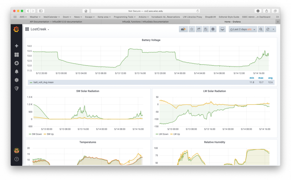
Figure 1 – Grafana dashboard for Lost Creek.
Database Creation
The database setup and data insertion are done using python. The python package influxDB-python is used to create and configure each database. I currently create a new database for each site. The time series data are grouped into different measurement types and then assigned different tags to provide a definition for the data. The two measurement types I define are “slowdata” and “fastdata.”
The minimum actions to create a database are to name it and apply a retention policy to the database. If you want to manipulate the data in the database automatically it is necessary to create continuous queries. InfluxDB-Python makes the creation of and management of the databases fairly easy.
Retention Policy
Two retention polices are created for long term (four weeks) and short term (one day) data storage. This retention policy uses about 1-2 Gb of disk storage for 20+ data streams. The high frequency flux data is stored for one day. This allows it to be down sampled to use less storage resources. It also allows you to view high frequency data if there appears to be some sort of anomaly. There is at least one default retention policy, in my code it is the one-day policy.
Continuous queries
Continuous queries act on the data in the influxDB database at a set time interval. In my case one-minute means are calculated from high frequency data fields in the “fastdata” measurement. The “fastata” fields are written into a new measurement “fastds4w.” The averaged data is then stored with the four-week long retention policy. There are no continuous queries that operate on the “slowdata.”
There is always the potential for irregular data arrival to the server so it is may be necessary to repeat a continuous query over a given interval. Currently, continuous queries are run every 30 minutes for three hours. This may not be optimal, but it seems to help insure that almost all of the “fastdata” is inserted into the “fastds4w” measurement in the database. Usually, failures of data showing up in the database are caused by cellular network connection issues and my simplistic methods for deciding what files are newly arrived in the directory.
Data insertion
InfluxDB-python has functions to insert Pandas dataframes into the database. I use a python script to read TOA5 data into a Pandas dataframe. This dataframe can be inserted directly into the database with influxDB-python functions. I find the influxDB-python functions very nice for interacting with the influxDB database. Previously, I used another method for inserting data into influxDB databases that worked but required more effort.
Setting up Grafana
Accounts are in hierarchical categories within Grafana, I’m not sure if this is the proper term. There are organizations and users. I have defined a single organization for all of my data sources and created users that are part of the organization. The organization/user structure is a bit confusing. If you don’t see what you expect when you are logged into you User account make sure that you are using the correct organization.
In order for Grafana to plot your data, you need to define a data source. Reading data from an influxDB database is included in Grafana and is accessed via an http connection. In my case it is a localhost connection since both applications are running on the same computer. Figure 2 shows the configuration page for setting up a data source. The configuration page is located in the gear icon on the left-hand panel.
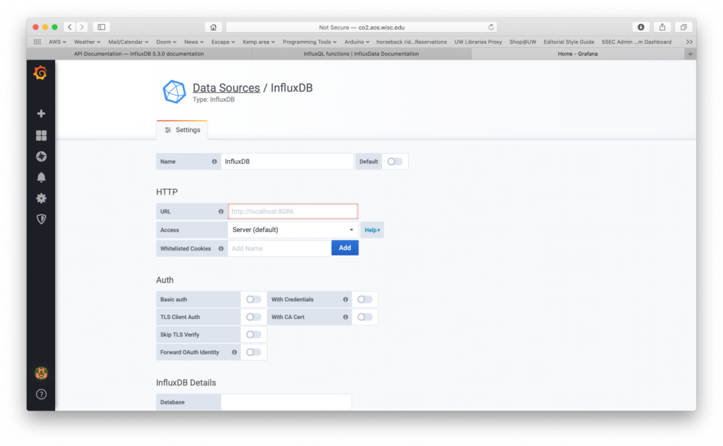
Figure 2 – Data source configuration screen. I connect to the database with http connection to port 8086.
Once you have defined your data source then you create a dashboard. The dashboard creation is located under the “+” symbol on the left-hand panel. I define each dashboard for each data stream. Once you create a dashboard, an empty canvas is created that you can add panels. Figure 3 shows the configuration tools to create a panel, specifically it shows the query tool for selecting what is plotted. You need to select the correct data source and then you can add fields to the plot. It is possible to include in each panels different statistics of the fields such as maximums, minimums and averages. The statistics operate over the time period selected.
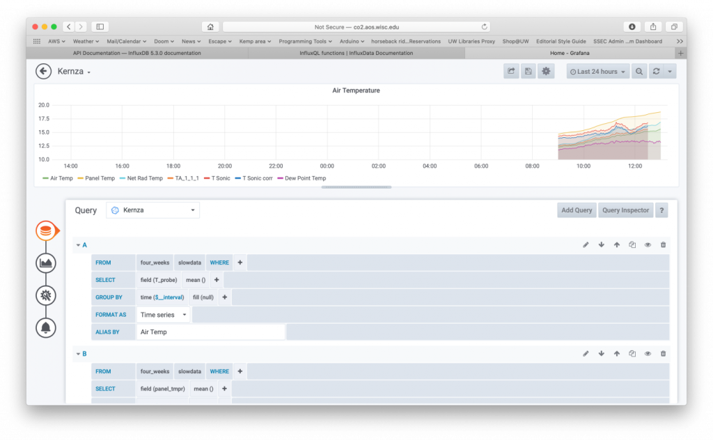
Figure 3 – Tools to set up a panel within a dashboard in Grafana.
Panels can include data plots, data tables, display webcam images, or print a data value. Here’s an example from Lost Creek: https://snapshot.raintank.io/dashboard/snapshot/Xtl4Ry7SrIVHf82dXlUXJYT12rIxnre3.
There are a lot of features in Grafana that I have not yet explored. I’ve gotten to a point where the system does what I need it to do. Grafana’s queries also do some averaging in its SQL queries, but this can also be configured. I have been experimenting with some of these features. This is another point where my database knowledge is limited.
Grafana has additional plug-ins that you can download as well. I currently use the windrose and plotly plugins. Plotly gives you the ability to create scatter plots.
Summary
The decision to use InfluxDB and Grafana came about because a colleague in the center where I work used it. There are other time series databases available that will work or be easier to implement. If you are already inserting data into a postgresql or mySQL database Grafana can read from those sources as well. There are some plotting features that are not available that would be nice to have such as contour plotting, but that is a minor complaint.
Overall, I have been very happy with the system and it has been running continuously for a number of years now. The methods to create databases and insert data into databases has evolved and been simplified over time.
Python Scripts
Files (*.zip) are available for download. Description of files below:
- campbellread_v2_0.py: function to read TOA5 files and put data into a Pandas dataframe.
- db_tools.py: functions to create database from TOA5 file, do some data quality control or add calculated fields to dataframe, and write data to the database.
- db_config.py: function to create field definitions for database.
- diagdecode.py: decodes Campbell and Licor diagnostic codes.
- insertWLEF.py and insertKernza.py: two functions that are run by cron to insert data into the database.
No Comments
Be the first to start a conversation