
This post was authored by Camilo Rey-Sanchez (current PostDoc at UC Berkeley, Biomet Lab) for the AmeriFlux Year of Methane.
If you have done chamber measurements of methane (CH4) flux in wetlands, you have probably noticed a high spatial heterogeneity in your data. If you are lucky, you have gone further to identify certain locations where your chamber measurements always tend to be higher. Some people have identified these places as “hotspots” of CH4 flux. In partially flooded systems such as pastures or grasslands, these hotspots may be associated with water pools that create the anaerobic conditions necessary for methanogens to produce CH4. In fully flooded ecosystems such as marshes or estuaries, these hotspots are sometimes associated with mudflats or places where the water level is very close to the surface (e.g. Rey-Sanchez, 2018).
This makes sense since a lower water table generally reduces oxidation of CH4 within the water column, thus allowing more CH4 to escape to the atmosphere. On other occasions, such as in my latest experience in an Ohio peat bog while pursuing my Ph.D., hotspots of CH4 emission are located in areas with no particular relationship to the water table (Rey-Sanchez, 2019). These hotspots exist rather due to a combination of factors, including the water level, the pH, the existence of other electron acceptors, the availability of labile carbon, or as I show in the paper referenced above, the ratio of methanogens to methanotrophs at the top of the peat. Although it is hard to say what exactly is creating these hotspots, I think that determining their existence within other wetlands is an interesting research endeavor to tackle, and one of the best ways to detect these hotspots is through eddy-covariance measurements and footprint modeling.
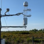
Eddy covariance (EC) measurements provide half-hourly measurements of CH4 flux that originate in a certain area around the tower, which we call the footprint. Its position around the tower is dependent on wind direction while its extension depends on turbulence conditions and atmospheric stability. In a short tower such as the one in Fig. 1, it can extend for hundreds of meters on a stable evening with calm winds, or to just 40-50 m if the atmosphere is highly unstable. The footprint model has been commonly used to filter data from unwanted locations, to evaluate the maximum extent of the sources, and more recently to evaluate the heterogeneity of sources within the footprint.
Researchers at the Biomet Lab at UC Berkeley where I am currently doing my postdoc have found that over a peatland pasture large CH4 emissions at night can be explained by hotspots captured by the long nighttime footprint (Baldocchi et al., 2012). Similarly, footprints from multiple towers have been used to parse the variability between open water and emerging vegetation zones within our wetlands (Matthes et al., 2014). One of my research objectives is to continue advancing our understanding of the spatial heterogeneity in CH4 fluxes by resolving details related to the location and magnitude of CH4 hotspots using the footprints, and to achieve this objective it is important that we use the best available tools in footprint modeling. Several footprint models exist that are based on parameterizations of Lagrangian stochastic models or solutions to the advection-diffusion equation. Although there have been several evaluations of these models, authors have pointed out the need for further evaluations under different atmospheric conditions. In addition, there have not been many evaluations of these models geared towards evaluating long-range footprints useful in identifying CH4 hotspots. With this motivation in mind, the biometeorology lab at UC Berkeley has collaborated with the Ameriflux team to deploy a tracer release experiment in one of our EC sites: An Alfalfa field on Bouldin Island in the Sacramento San Joaquin River Delta (Fig 1).
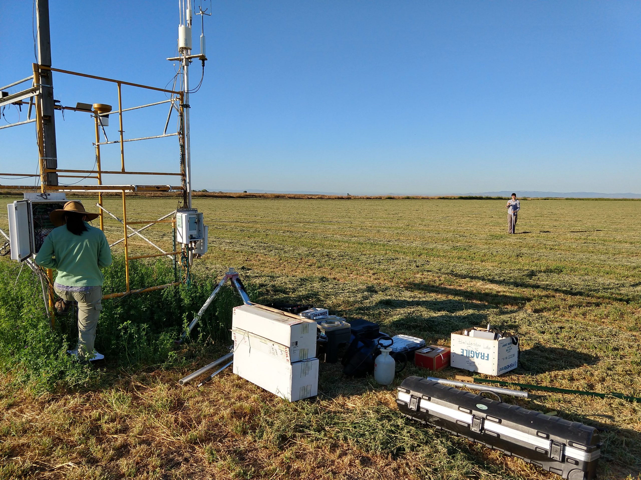
Figure 1. Our site in Bouldin Island (US-Bi1) shortly after the Alfalfa was mowed. Daphne Szutu (left) downloads data and Camilo Rey (right) measures the distance and direction for the tracer release. Photo by Housen Chu.
The Alfalfa field on Bouldin Island provides a perfect scenario to validate footprint models because it is a very flat site, homogeneous, with steady winds and long fetch, and with a near-zero CH4 flux. Moreover, we can freely move within the field and locate tracer sources in different directions and distances upwind from the tower. By knowing the flow rate of our CH4 tracer as well as the distance and direction from the tower, we can compute a flux through the footprint model and compare that to the measurements of our EC system.
There have been two tracer gas release campaigns. In the first one, the tracer gas was released through a 10 ft pipe with 5 outlets at different flow rates and distances from the tower. This initial evaluation allowed us to determine the minimal flow rates and distances needed to obtain a strong signal in the EC measurements.
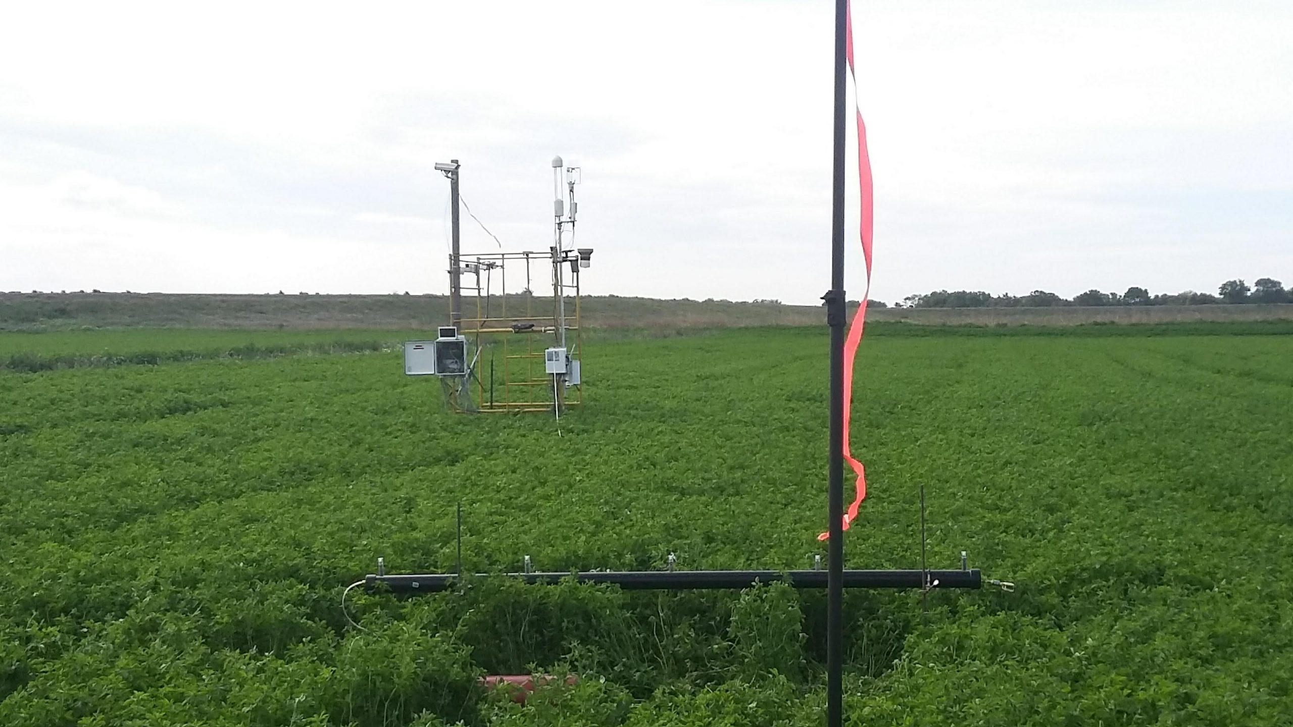
Figure 2. The initial release at 20 m from the tower. The pink ribbon helped us confirm the direction of the wind, which thankfully was more or less consistent throughout the day. Photo by: Camilo Rey.
For the second campaign, we set for a longer release that would allow us to collect more data points and encompass different atmospheric conditions. For this second campaign, we included one release point at 20 m from the tower that was activated only during the daytime, and a second release point at 180 m from the tower activated only during nighttime hours. Fig 3 shows the first release point, which was activated only at daytime through a solenoid valve.

Figure 3. Daytime release located 20 m from the tower. The solenoid valve was activated with a Campbell data logger (CR10), and the valve and data logger were powered by a battery connected to a small solar panel. Photo by Housen Chu.
Thanks to the Ameriflux Tech team, a secondary tower was deployed at a lower height, thus allowing a second data set to validate the fluxes from the release point.

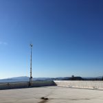
Figure 4. Joe Verfaillie from the Biomet lab sets up the secondary tower and ancillary measurements
This secondary tower doubles the number of points for the validation of footprints. In addition to this, we also installed a sonic anemometer at a third level, 60 cm above the ground, which will allow us to obtain a three-point wind profile and thus improve the current estimates of roughness length and displacement height necessary for these footprint models.
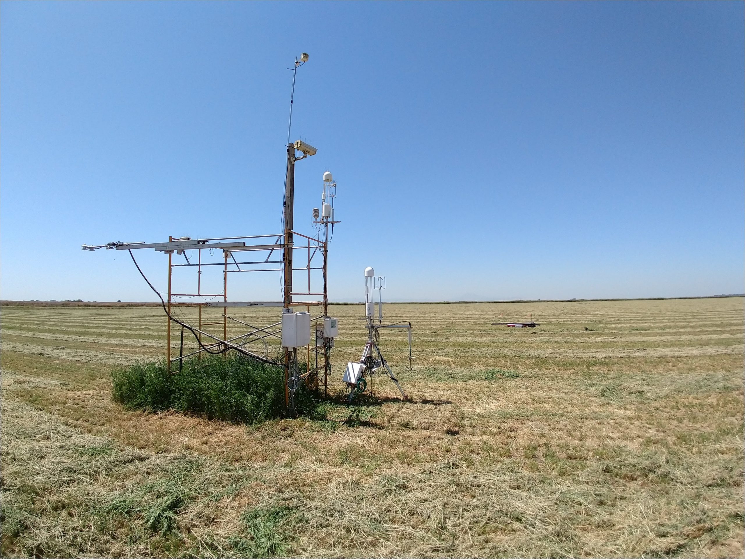
Figure 5. Final setup of the tracer release experiment with two levels of gas exchange measurements and a lower level with additional wind measurements.
We are currently testing three commonly used footprint models (Hsieh et al., 2000; Kljun et al., 2015; Kormann & Meixner, 2001), and have included a nighttime release to validate the nighttime footprints. Given that nighttime footprints tend to extend much longer than daytime footprints, this is essential for the detection of long-range hotspots. Detecting hotspots of CH4 is important for analyzing the different biogeochemical and physical processes that lead to these high emissions. Moreover, representing hotspots in CH4 models has the potential to improve current gap-filling techniques in eddy covariance measurements, especially on sites where there is high spatial heterogeneity in CH4 emissions.
Some of the outcomes from this tracer release experiment will aid to 1) Understand what footprint models are more suitable for our sites; 2) Study the role of static stability in the discrepancies between prediction and measurements; 3) Identify the best model to detect long-range emissions where potential hotspots of CH4 can be found; 4) Provide recommendations for researchers interested in downscaling footprints to understand the spatial heterogeneity of their fluxes; and 5) create a framework for the inversion of these models to detect magnitudes and dimensions of hotspots, especially if dual flux towers are used in the future.
References
Baldocchi, D., Detto, M., Sonnentag, O., Verfaillie, J., Teh, Y. A., Silver, W., & Kelly, N. M. (2012). The challenges of measuring methane fluxes and concentrations over a peatland pasture. Agricultural and Forest Meteorology, 153, 177–187. https://doi.org/10.1016/j.agrformet.2011.04.013
Hsieh, C. I., Katul, G., & Chi, T. (2000). An approximate analytical model for footprint estimation of scaler fluxes in thermally stratified atmospheric flows. Advances in Water Resources, 23(7), 765–772. https://doi.org/10.1016/s0309-1708(99)00042-1
Kljun, N., Calanca, P., Rotach, M. W., & Schmid, H. P. (2015). A simple two-dimensional parameterisation for Flux Footprint Prediction (FFP). Geoscientific Model Development, 8(11), 3695–3713. https://doi.org/10.5194/gmd-8-3695-2015
Kormann, R., & Meixner, F. X. (2001). An Analytical Footprint Model For Non-Neutral Stratification. Boundary-Layer Meteorology, 99(2), 207–224. https://doi.org/10.1023/A:1018991015119
Matthes, J. H., Sturtevant, C., Verfaillie, J., Knox, S., & Baldocchi, D. (2014). Parsing the variability in CH4 flux at a spatially heterogeneous wetland: Integrating multiple eddy covariance towers with high-resolution flux footprint analysis. Journal of Geophysical Research: Biogeosciences, 119(7), 1322–1339. https://doi.org/10.1002/2014JG002642
Rey-Sanchez, A. C., Morin, T. H., Stefanik, K. C., Wrighton, K., & Bohrer, G. (2018). Determining total emissions and environmental drivers of methane flux in a Lake Erie estuarine marsh. Ecological Engineering, 114, 7–15. https://doi.org/10.1016/j.ecoleng.2017.06.042
Rey-Sanchez, C., Bohrer, G., Slater, J., Li, Y.-F., Grau-Andrés, R., Hao, Y., et al. (2019). The ratio of methanogens to methanotrophs and water-level dynamics drive methane transfer velocity in a temperate kettle-hole peat bog. Biogeosciences, 16(16), 3207–3231. https://doi.org/10.5194/bg-16-3207-2019

No Comments
Be the first to start a conversation